Tight Spans of Finite Metric Spaces
Introduction
To each finite metric space M one can assign a polyhedral complex which captures essential features of M, the tight span T(M). This name was introduced by Bandelt and Dress [1], but these objects already showed up earlier as the injective envelope of a metric space in the work of Isbell [12].
The probably easiest examples of finite metric spaces are the tree-like ones: Just take a finite tree, that is, a connected graph without cycles with non-negative weights (or lengths) assigned to the edges. We want to define a metric space on the nodes of the tree. Since shortest paths between any two nodes in a tree are unique, the lengths on the edges define a metric.
Being the bounded subcomplex of an unbounded polyhedron, T(M) is necessarily contractible. Hence, T(M) is one-dimensional if and only if T(M) is a tree. Moreover, if M is tree-like then T(M) is a metrically correct copy of the tree which defined M. In a way, T(M) can be seen as the space of all possible trees which fit best to M.
Interesting examples of finite metric spaces arise in computational biology, more precisely in phylogenetics, as follows: Starting out with a bunch of DNA sequences of individual plants or animals (called taxa) these DNA sequences are first aligned such that it is then possible to compute the (editing) distance between any two taxa. This distance function is only slightly more sophisticated than counting the non-matching bases in the aligned DNA sequences. It naturally defines a finite metric space.
The phylogenetic problem is to (re-)construct the genealogy of a set of taxa. Tight spans now provide one approach to the phylogenetic problem. They are particularly useful to find out whether or not there exists a meaningful tree which explains the metric data.
An Example
Let us consider six species of bees of which are given by (very short) fragments of already aligned DNA data. On purpose, in fact, only 677 bases were taken. The (symmetric) editing distance matrix looks as listed below. The picture of the honeybee (apis mellifera) on the right is taken from Wikipedia..jpg)
.jpg)
The Distance Matrix
| A.andrenof | A.mellifer | A.dorsata | A.cerana | A.florea | A.koschev | |
| A.andrenof | 0.0 | 0.090103395 | 0.10339734 | 0.09601182 | 0.0044313148 | 0.07533235 |
| A.mellifer | 0.090103395 | 0.0 | 0.09305761 | 0.090103395 | 0.09305761 | 0.10044313 |
| A.dorsata | 0.10339734 | 0.09305761 | 0.0 | 0.116691284 | 0.106351554 | 0.10339734 |
| A.cerana | 0.09601182 | 0.090103395 | 0.116691284 | 0.0 | 0.098966025 | 0.098966025 |
| A.florea | 0.0044313148 | 0.09305761 | 0.106351554 | 0.098966025 | 0.0 | 0.07828656 |
| A.koschev | 0.07533235 | 0.10044313 | 0.10339734 | 0.098966025 | 0.07828656 | 0.0 |
This data set stems from the example file bees.nex of the SplitsTree program of Huson and Bryant [11]. The names of the bees (apis ...) are truncated to eight characters.
The Tight Span of Six Bees
It is important to keep in mind that the tight span, in general, is a high-dimensional geometric object which may be very difficult to visualize properly; see [6] for suggestions.
Our software system polymake allows to deal with and to compute tight spans [6]. Further it can also visualize tight spans by feeding suitable input to various viewers. However, as already disclaimed in the previous paragraph, these images need a bit of explanation. Here is a polymake (version 3.0) file describing the tight span of the six bees. Only the sections METRIC and TAXA are provided as input; the rest is computed by polymake.
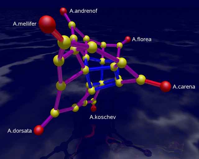
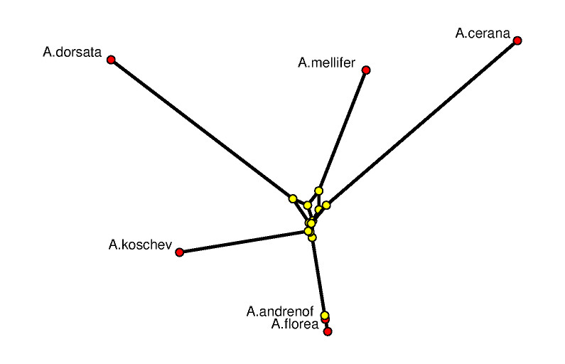
The picture on the left shows a 3-dimensional rendering of the tight span in a way such that its combinatorial features are emphasized. In particular, it is a difficult image to derive biological information from. The picture is produced with POV-RAY via polymake. The picture on the right tries to be metrically as correct as possible. See [7] for the visualization aspects of the subject.
The combinatorial output is obtained via polymake's function VISUAL_BOUNDED_GRAPH, while the metric output comes from VISUAL_TIGHT_SPAN. In both cases the red points are vertices of the tight span related to taxa, while the yellow ones are non-taxon vertices. In a successful phylogenetic reconstruction they might biologically be interpreted as common ancestors.
The edge colors in both combinatorial outputs indicate the maximum dimension of a bounded face containing that edge. The more blue the edge the higher the dimension. In an example with six taxa, the tight span is either 2-dimensional or 3-dimensional (this was shown by Develin [3]). Our bee related tight span here is 3-dimensional. A red edge means that there is no bounded face of higher dimension containing this edge, purple indicates that there is a 2-face but not no 3-face containing the edge, and blue means that there is a 3-face containing this edge.
The following can be read off the metric picture: The data suggests that A.florea descends from A.andrenof, while all other relationships are more distant. The little amount of phylogenetic information to be retrieved here is due to the fact that we started out with extremely short DNA fragments. This example was chosen on purpose since it shows how tight spans can locate that part of the genetic information which really is tree-like.
Extensions
A key result on the structure of finite metric spaces and their tight spans is the Split Decomposition Theorem of Bandelt and Dress [2]. It says that each metric on a finite set of taxa can be written as the sum of so-called split metrics (which induce a partition of the taxa into exactly two sets) and an indecomposable rest.
It turns out that finite metric spaces can be described in terms of polyhedral geometry as the regular subdivision of a second hypersimplex [13]. In this way the Split Decomposition Theorem has a natural generalization where the (vertices of the) second hypersimplices are replaced by arbitrary point configurations, see [9] and [10]. This is relevant, e.g, for applications in tropical geometry [8].
References
- H.-J. Bandelt and A. Dress: Reconstructing the shape of a tree from observed dissimilarity data, Adv. in Appl. Math. 7 (1986), no. 3, 309-343.
- H.-J. Bandelt and A. Dress: A canonical decomposition theory for metrics on a finite set, Adv. Math. 92 (1992), 47-105.
- M. Develin: Dimensions of tight spans. Ann. Comb. 10 (2006), no. 1, 53-61.
- A. W. M. Dress: Trees, tight extensions of metric spaces, and the cohomological dimension of certain groups: a note on combinatorial properties of metric spaces, Adv. in Math. 53 (1984), no. 3, 321-402.
- A. W. M. Dress, K. T. Huber, and V. Moulton: A comparison between two distinct continuous models in projective cluster theory: the median and the tight-span construction, Ann. Comb. 2 (1998), no. 4, 299-311.
- E. Gawrilow and M. Joswig: polymake: a framework for analyzing convex polytopes, Polytopes---combinatorics and computation (Oberwolfach, 1997), 43-73, Birkhäuser, Basel, 2000.
- E. Gawrilow, M. Joswig, T. Rörig, and N. Witte: Drawing polytopal graphs with polymake. Comput. Vis. Sci. 13 (2010), no. 2, 99-110.
- S. Herrmann, A. Jensen, M. Joswig and B. Sturmfels: How to draw tropical planes, The Electronic Journal of Combinatorics 16(2) (2009), #R6
- S. Herrmann and M. Joswig: Splitting polytopes. Münster J. Math. 1 (2008), 109-141.
- H. Hirai: A geometric study of the split decomposition. Discrete Comput. Geom. 36 (2006), no. 2, 331-361.
- D. H. Huson and D. Bryant, Application of Phylogenetic Networks in Evolutionary Studies, Mol. Biol. Evol., 23(2):254-267, 2006.
- J. R. Isbell: Six theorems about injective metric spaces, Comment. Math. Helv. 39 (1964), 65-76.
- B. Sturmfels and J. Yu: Classification of six point metrics, The Electronic Journal of Combinatorics, 11 (2004), #R44. Website